Building a metrics backend (time series db) with PostgreSQL and Rust

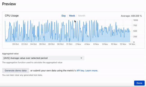
At ilert customers are already benefitting from our easy to setup private or public status pages and auto generated SLA uptime graphs for their business services. However, we decided to push the graph topic a bit further with custom metrics. Using ilert metrics customers can showcase additional business data and insights into their services on their status pages.

To ingest, store, query and aggregate metrics (time series) data we looked at the solutions out there, especially the solutions of cloud providers; but in the end decided to model our own time series database using the tools we already know and rely on while fitting them perfectly onto our specific use case and reducing complexity and hosting costs.

This post describes the development of a time series database ditching fancy cloud solutions for well known and proven tools: PostgreSQL and Rust (diesel + actix) - read more about the reasons below.

Why use Rust?

Rust has grown in popularity over the years and is used in many different areas of programming such as game development, microcontroller applications and even web development.

A major difference between other lower-level programming languages like C/C++ is the memory management, which includes features such as ownerships, the borrow checker and lifetimes, helping developers to prevent memory violation errors. These bugs will be detected at compile time. In addition the running process doesn’t require a garbage collector unlike in Java or C#. High performance while processing large amounts of data and the support for concurrent programming using tokio is a great benefit when it comes to our use case of creating and running a time series database.

At ilert we also love the fact that Rust enables us to ship ervice artifacts with an extremely small footprint. Service docker images usually do not exceed 20MB and memory consumption of our services (depending on load) is super efficient keeping required RAM often below 10MB. This allows us to scale containers and balance load across multiple Kubernetes clusters with a focus on high availability and ignore the cost factor of running so many containers.

Why use PostgreSQL?

PostgreSQL is an open source object-relational database system with the capacity to use and extend the SQL language while combining many features to safely store and scale the most large complex data workloads.

Coming from a MySQL background, one of the most useful features of PostgreSQL when creating a time series database is the ability to use arrays and multi-dimensional arrays, which allows us to store and assign multiple values to a “time container” in a single row.

Ingestion stack, controlling the time series data flow

Following diagram illustrates the ingestion process:

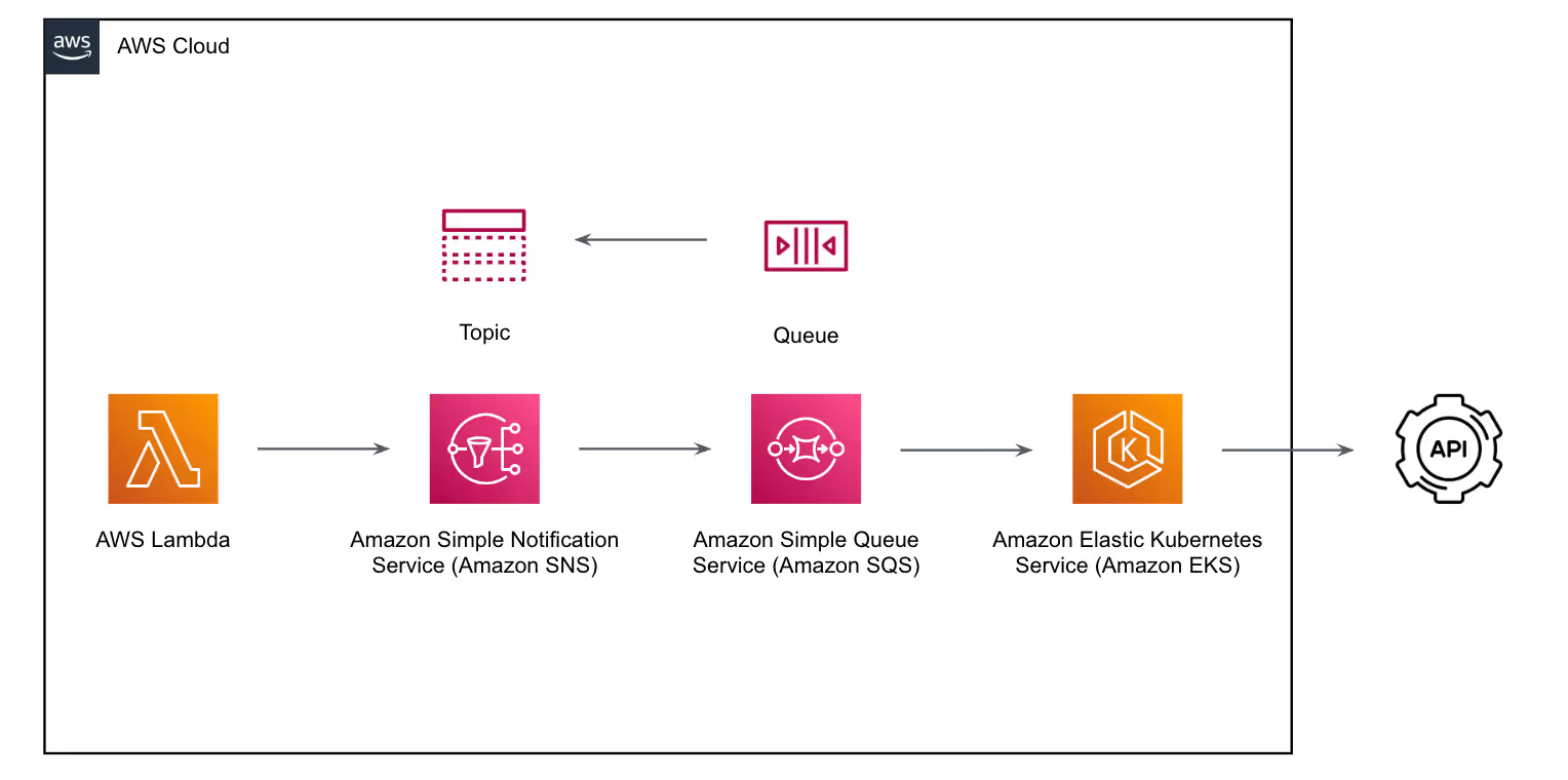
We use AWS Lambda to validate and authenticate incoming time series data and pipe it to AWS SNS (Simple Notification Service), which then pipes to AWS SQS (Simple Queue Service). Our Rust service which is deployed on AWS EKS (Elastic Kubernetes Service) will consume the messages from the queue and process them to be stored in our PostgreSQL database.

The whole serverless inbound ingestion queue stack ensures that we can easily scale and helps us control the incoming flow of time series data. We can individually scale the Rust service and Postgres instances behind the queue to match input pressure with output consumption.

A simplified version of such a message looks like this:

{
  "metricId": 1,
    "series": [
      {
        "timestamp": 1663160400,
        "value": 0.02
      }
    ]
}

Storing and partitioning time series data

Consuming the message described above, one could simply decide to store each series value in a row.

create table time_series {
  id bigint not null,
  ts bigint not null,
  series double precision,
  primary key(id, ts)
}

However when scaling this out to hundred thousands of metrics we need to deal with billions of rows. Storing a single value per second per month for a single metric already leaves us with 2 678 400 rows.

By introducing a “container” that spans over a certain window e.g. 1 hour we could already reduce the amount of rows by a factor of 60 landing at just 44 640 rows:

create table time_series {
  id bigint not null,
  ts bigint not null,
  series double precision[][],
  primary key(id, ts)
}

How do we achieve this? There are two main things to do here.

1. Turn our series column into a multi dimensional array series double precision -> series double precision[][] storing the timestamp on the left and the value on the right.
2. Truncate the incoming series timestamp on the base of our container size for incoming series data to find the right place to append the array

fn round_epoch_to_interval(time_sec: i64, interval_sec: i64, round_up: bool) -> ILertResult {

    let offset = time_sec % interval_sec;
    let rounded = time_sec - offset;

    let result = if offset > (interval_sec / 2) {
        if round_up {
            rounded + interval_sec
        } else {
            rounded
        }
    } else{
        rounded
    };

    Ok(result)
}

But there is more.

What if we do not need second or even millisecond precision for our use case?

Imagine a graph showing a month of data points in a few hundred pixels wide on a mobile device. There is no way that we could fit 44640 let alone 2678400 data points in there.

We found that the sweet spot is somewhere between 250-500 data points for such a graph. Therefore further grouping through secondary truncation was possible.

In the end we wanted to be flexible and designed the precision (truncation level 1 and 2) to be dynamic so that we can adjust it anytime to match different use cases.

However we decided to use 30 seconds as default value, meaning that we store 2 data points per minute per metric.

The second grouping works by not only truncating the series timestamp to the container (row.ts) e.g. 1 hour but also truncating it a second time to the index of the left array (row.series[i][]) e.g. 30 seconds. This gives us a maximum size for the arrays of each to work with 3600 / 30 = 120.

Caveats

But this design does come with its caveats, we cannot simply run an INSERT INTO time_series statement to store data anymore. We need to know whether we have to create a new container (row) if it does not exist yet. Additionally if you were to decide that it should be possible to overwrite existing timepoints, which we wanted to make possible, you would also need to know whether to add the data point to the array or overwrite an already existing entry - also, the array does not guarantee order anymore meaning we have to keep that in mind when querying the data.

To understand what needs to be done for each time series point, we open a transaction and run a query similar to this:

select array_position(ARRAY(SELECT unnest(series[:][1])), 1663160400) as pos -- truncated 30
from timeseries
where id = 1
and ts = 1663160400 -- truncated 3600
FOR UPDATE

Note: FOR UPDATE will lock the row in case it exists

Depending on the result we will know if we have to:

1. Create a new row for this hour (truncated 3600) container insert into timeseries values (1663160400, 1, '{{1663160400, 0.02}}')
2. Append a new time series value to the existing row array update timeseries set series = series || '{1663160400, 0.02}
3. Overwrite an existing index in the row’s array with a new value update timeseries set series[1663160400][2] = 0.02

Fetching and aggregating time series data

Before looking at the specific SQL to query time series data, let us have a look at the REST interface used by other services to access time series data.

curl https://host:6969/metrics/1/series?aggregation=avg&from=1666000302&until=1668678702&interval-sec=8064

• from and until are quite self explanatory, we need to provide a range for which we want to fetch the data e.g. the last 28 days
• aggregation will always be applied when querying data and the default is avg - average
• interval-sec always required, describes the window size for the aggregation

interval-sec is where the magic happens for our query, we already stated above that a sweet spot for a graph display is somewhere between 250-500 data points and with us storing a time point about every 30 seconds we still have a lot more points than that (80640) in a months view. Using this window size in seconds we can let PostgreSQL further aggregate our time series data to the desired amount time points for our graph.

Our query then works in roughly four parts, it will:

1. Query the hourly containers (rows) that fit to the provided from and until time range (truncation for input is needed here to work accurately)
2. Use PostgreSQL unnest() to convert our array items into row results
3. Group by truncated interval-sec, while aggregating
4. Ensure order of timestamps

A simplified sample of a query that would be build for our HTTP request above would look like this:

select extract(epoch from date_trunc('day', sub.ts))::bigint as container,
(extract(hour FROM sub.ts)::int / 2) AS agg_slot,
avg(sub.val) AS agg_val
from
(select to_timestamp(unnest(series[:][1:1])) as ts, unnest(series[:][2:2]) as val
from timeseries where id = 1 and ts >= 1666000302 and ts <= 1668678702) sub
where sub.ts >= to_timestamp(1666000302) and sub.ts <= to_timestamp(1668678702)
group by container, agg_slot
order by container, agg_slot asc

Note: based on the interval-sec values for date_trunc() and extract() are build to create dynamic but deterministic grouping windows (called slot in the SQL statement), the resulting rows will not contain timestamps but relativ values to these slots, the Rust code will then rebuild the timestamps based on the results and input parameters

let ts = (row.container +
  (Dao::slot_to_seconds(slot_size.as_str())? // hour => 3600
      * (row.agg_slot as i64)
      * slot_value));

A sample result for the query above would look like this after all result rows have been processed into a JSON response:

{
  "aggregation": "avg",
  "totalAgg": 0.02,
  "series": [
    [
      1666000302,
      0.02
    ],
    [
      1666008366,
      0.02
    ],
    // ...
  ]
}

Zooming out

In software development new frameworks, libraries or in this case databases are not always needed or better when use cases are properly identified and understood. Often solutions based on the existing stack can be kept simpler and implemented without increasing the complexity of the stack as whole.

There are even further benefits when integrating a solution like this on a known concept, as the other parts of the existing ecosystem already integrate with them, in our case this relates to:

• Performance and insight metrics
• Business metrics
• Logging
• Scaling (k8s)
• Compliance & GDPR
• Monitoring
• Alerting
• Build pipelines (CI & CD)

If you want to try out metrics and the time series API in action, feel free to play around with it in your very own ilert account: It is free.

If you want to learn more about how we build microservices, time series databases or alerting platforms in Rust at ilert reach out to us

We are hiring :)

‍